Personal reflections on Stat the Landing

In this week’s exercise we were tasked by the FAA to understand the distribution, characteristics, and components of individual airports operations that are leading to increased delays.

My first step was to identify which airports are the “problem children.”

My plan was to use clustering on PCAs to show what airports have higher than normal delay times and whose operations have been flat or worsening.

Once I identified what airports are the problems we can figure out what they have in common.

Methodology

I’ve found that for most projects there have been data that would be useful to pull in externally as well as superfluous data in the files supplied. This case was no different.

I chose not to bring in external data for this project, however. This was a hard choice to make, since I always want to make the most robust model I can and there were many external agents that could impact delay times like weather, tourism, and service expansions (as indicated in the summary of the project)

The most important part of my approach to this project was that I only wanted to use current data, the latest being 2014, supplemented by a change score from prior years. This meant that I would be using far fewer data than others in the class, but I felt that it would have more significant results and would be more of a “real world” approach.

This approach ended up causing me a good deal of frustration. I assumed that having fewer data would simply show the cluster and principle component patterns with less noise, but they really just made both very sparse and difficult to differentiate. I ended up biting the bullet and taking data from 2012-2014. I decided that this would still give me current data while actually mellowing out any particularly bad years.

The results I got suggested that I really could use another couple of years in there, but I decided that the approach was correct and I would be able to work with it without diluting it further.

Correlations

One of the questions asked in the project was the value of correlations in PCA. I had gone in assuming that you could use them similarly as in other analyses, eliminating colinear or entirely extraneous features. I did a fairly exhaustive review of this, though, and found that using correlation this way really had no impact.

Checking for pairs with correlations >.95. Will exclude the one of the pair with the greater sum of absolute correlations for all features (the one that has more of its explanatory power already covered by other features). If there is a tie (or close to) I’ll favor delays over arrivals.

• A - Departure Cancellations and Arrival Cancellations .999 correlated, dropping Arrival Cancellations
• B - Deparetures for Metric Computations and Arrivals for Metric Computations .999 correlated, dropping Arrivals
• C - Average Airport Departure Delay and Percent on-time airport departures -.96 correlated, dropping Average Airport Departure Delay
• D - Average Gate Arrival Delay and Percent on-time gate arrivals -.95 correlated, dropping Percent on-time Gate Arrivals.

Had first done this naive–none of the above exclusions.

After doing this my cumed eigenvalues declined. Testing to see whether I should have done different exclusions if any.

• Naive
• i. ABCD excluded
• ii. ABC excluded
• iii. ABD excluded
• iv. ACD excluded
• v. BCD excluded
• vi. inverse ABCD (excluded the other partner in the pair)
• vii. iABC excluded
• viii. iABD excluded
• ix. iACD excluded
• x. iBCD excluded

Data: Cum PC1 / PC2 / PC3

• 36 / 66 / 82
• i. 37 / 62 / 79
• ii. 34 / 64 / 80
• iii. 37 / 64 / 80
• iv. 40 / 64 / 80
• v. 38 / 62 / 80
• vi. 37 / 62 / 80
• vii. 35 / 64 / 81
• viii. 36 / 65 / 81
• ix. 41 / 64 / 80
• x. 38 / 62 / 81

From this analysis I can see that dropping factors based on correlation is actually harmful and that I had been targeting the wrong member of the correlated pairs.

As a last test I’ll look at dropping only one of the inverse members at a time:

• dropping iA: 36 / 67 / 81
• dropping iB: 35 / 65 / 82
• dropping iC: 38 / 64 / 81
• dropping iD: 38 / 65 / 81

So it looks like excluding for correlation is the wrong way to go.

PCA and Clustering

It turned out that some highly correlated pairs proved to have great impact on the PCA. I was also happy to see that the change metrics I created were also important contributors.

It was in this point in the process that I decided that I’d needed to bring in 2012-2014.

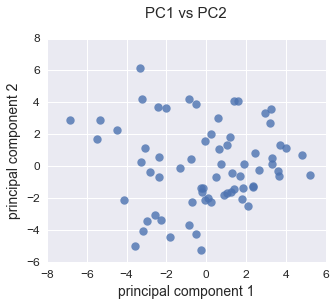
PCA with 2014 Only

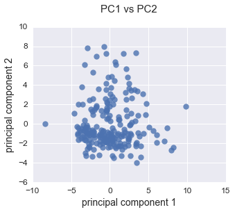
PCA with 2012-2014 Only

Once I had these principle components locked down, it was time to cluster the airports. I started with DB-SCAN, but that really didn’t give me satisfactory results, 2 clusters with a -.283 Silhouette.

So I went K-Means, trying it with Ks of 2, 3, and 4. 3 was easily the best choice.

The rest of the project’s results can be seen on its main page.

Personal Take-aways

This was probably my favorite project so far. That’s not because it was the most riveting topic or the most robust data set or having the most tools available to me.

A lot of it is the amount of time I spent on it, despite having to be done around challenging circumstances. I think that in past projects I have had this terrible sense of conflict between wanting to really submerge myself into the work and wanting to get it done on time. On this project I was told that I could take more time with it and it really helped terrifically. I know that this isn’t something that often happens in the real world, but it was really useful here.

I also really enjoy that I came to a clear answer. That’s also not something that often happens in the real world. There’s always a range of possibilities, but given the data at hand, when there was so much else I could theoretically have used to bolster it, it was amazing to say, “here it is, the source of the problems.”